Linear regression – learning algorithm with Python

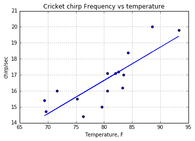
In this post, we will demystify the learning algorithm of linear regression. We will analyze the simplest univariate case with single feature X wherein the previous example was temperature and output was cricket chirps/sec. Let’s use the same data with crickets to build learning algorithm and see if it produces a similar hypothesis as in excel.

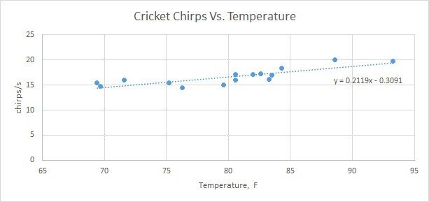
As you may already know from this example, we need to find linear equation parameters θ₀ and θ₁, to fit line most optimally on the given data set:

y = θ₀ + θ₁ x

x here is a feature (temperature), and y – output value (chirps/sec). So how are we going to find parameters θ₀ and θ₁? The whole point of the learning algorithm is doing this iteratively. We need to find optimal θ₀, and θ₁ parameter values, so that approximation line error from the plotted training set is minimal. By doing successive corrections to randomly selected parameters we can find an optimal solution. From statistics, you probably know the Least Mean Square (LMS) algorithm. It uses gradient-based method of steepest descent.

First of all, we construct a cost function J() which calculates the square error between suggested output and real output:

We need to minimize J(θ0, θ1) by adjusting θ0, θ1 parameters in several iterations. First of all we need to find derivatives of the cost function for both theta parameters. And then update each parameter with some learning rate α.

Repeat until converge {

}

Without proof gradient descent algorithm has to perform following update for every theta:

Repeat until converge{

}

As you will see on every iteration, θ0 and θ1 parameters on each iteration will get closer and closer to optimized values by finding the local minimum in cost function J. For this example, we will initiate α parameter and number of iterations by intuition.

In this and future examples, I am going to use Python-based environment. For Windows users, it is best to download Anakonda package, which already includes latest Python release, SciPi, and other 400 popular Python packages, including special machine learning tools (which we might use in future). It is open source so everyone can get hands on it. It is pretty new to me, so this will be a learning process for me too. It also comes with powerful GUI spyder.

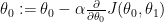
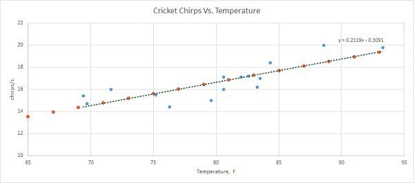
Let us start writing Python programs gradually. First of all, we need to read cricket data from the file. I have saved it as CSV from Excel:

The first column is an output (Y), and second is inputs/features (X).

First of all, we need to write a couple of functions: cost and gradient_descent:

def cost(x,y,theta):
    m = y.size #number of training examples
    predicted = x.dot(theta).flatten()
    sqErr = (predicted - y) ** 2
    J = (1.0) / (2 * m) * sqErr.sum()
    return J
def gradient_descent(x, y, theta, alpha, iterations):
#gradient descent algorithm to find optimal theta values
    m = y.size
    J_theta_log = np.zeros(shape=(iterations+1, 3))
#store initial values in to log    
    J_theta_log[0, 0] = cost(x, y, theta)
    J_theta_log[0,1] = theta[0][0]
    J_theta_log[0,2] = theta[1][0]
   # theta_log = np.zeros(shape=(iterations,2))
    for i in range(iterations):
#split equation in to several parts
        predicted = x.dot(theta).flatten()

        err1 = (predicted - y) * x[:, 0]
        err2 = (predicted - y) * x[:, 1]

        theta[0][0] = theta[0][0] - alpha * (1.0 / m) * err1.sum()
        theta[1][0] = theta[1][0] - alpha * (1.0 / m) * err2.sum()

        J_theta_log[i+1, 0] = cost(x, y, theta)
        J_theta_log[i+1,1] = theta[0][0]
        J_theta_log[i+1,2] = theta[1][0]

    return theta, J_theta_log

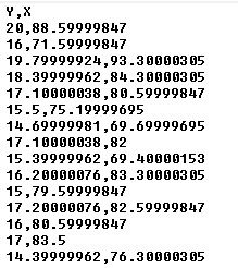
In gradient_descent function, we also save cost and theta values to show in the graph how they travel towards minimum point.

After less than 20 iterations, we already got a local minimum point:

Machine-learned linear regression hypothesis looks like:

y = 0.0026 + 0.2081 • x

And this is how it looks on the training data graph:

And the final test is to run a hypothesis with some test data:

At temperature = 85F, predicted chirp frequency 17.687319

At temperature = 50F, predicted chirp frequency 10.405367

You may notice that machine-learned formula parameters are somewhat different from excel trend formula, but when you plot data on top of it, you can see that red dots lie on top of the trend.

We didn’t implement feature x normalization to reduce calculation overhead. But this is more applicable to learning with multiple features where we would like to make them similar in scale. Download python code here [linear regression.zip] to run in Anaconda.