
This is the simplest optimization routine. Using this algorithm, optimization parameters are changed separately in each step. Only one parameter can be changed in one step while others are held as constants.
Xk+1=Xk+ΔXk , k=0,1,2,…
ΔXk step of parameter Xk. The parameter is changed until function growth is noticed, and then the next parameter follows, and so on. After the cycle with all parameters is completed, the step is changed to half its value and repeats. Optimal point searching ends when there is no function increase, and the last point is held as an optimal point.
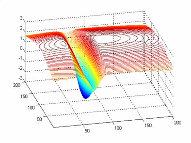
First function optimization example

Its plot:

Using the MATLAB script, we get the results below. In each picture, the start coordinates are different.
Start coordinates. x=150; y=200;

Start coordinates x=50; y=150;

Another example


Start coordinates x=10; y=10;

Start coordinates x=100; y=200;

The third example


Start coordinates x=50; y=200;

Matlab script
close all;
clear all;
clc;
[X,Y] = meshgrid(-100:1:100, -100:1:100);
Z =3*exp(-((X.^2)/78000) -((Y.^2)/20000))-5*exp(-(((X+31).^2)/123) -(((Y+20).^2)/5000));
xx=100;
yy=100;
contour3(Z,20);
hold on;
% figure(2); mesh(Z);
%  figure
%  plot3(X,Y,Z)
X=70; Y=100;
X1=0;Y1=0;
X0=X;
Y0=Y;
z=160; figure(1); plot(X,Y,'r*'), hold on;
 X=X-xx; Y=Y-yy;
TT1 =3*exp(-((X.^2)/78000) -((Y.^2)/20000))-5*exp(-(((X+31).^2)/123) -(((Y+20).^2)/5053));
for i=1:50

   z=z/2;
   X=X-z;
   Z2  =3*exp(-((X.^2)/78000) -((Y.^2)/20000))-5*exp(-(((X+31).^2)/123) -(((Y+20).^2)/5053));
   if Z2>=TT1
      TT=Z2;
      X1=X;
   end;
   X=X+(2*z);
   Z2  =3*exp(-((X.^2)/78000) -((Y.^2)/20000))-5*exp(-(((X+31).^2)/123) -(((Y+20).^2)/5053));
   if Z2>=TT1
       TT=Z2;
      X1=X;
   end;
    TT1=TT;
     X=X1;
    X=X+xx; Y=Y+yy;
   figure(1); plot3(X,Y,TT,'g*'), hold on;
   XX=[X0 X];
   YY=[Y0 Y];
   line(XX,YY, 'LineWidth',1); hold on;
   X0=X;
   Y0=Y;
   X=X-xx; Y=Y-yy;
   Y=Y+z;
   Z2 = 3*exp(-((X.^2)/78000) -((Y.^2)/20000))-5*exp(-(((X+31).^2)/123) -(((Y+20).^2)/5053));
   if Z2>=TT1
      TT=Z2;
      Y1=Y;
   end;
   Y=Y-(2*z);
   Z2 = 3*exp(-((X.^2)/78000) -((Y.^2)/20000))-5*exp(-(((X+31).^2)/123) -(((Y+20).^2)/5053));
   if Z2>=TT1
      TT=Z2;
      Y1=Y;
   end;
   TT1=TT;
   Y=Y1;
   X=X+xx; Y=Y+yy;
   figure(1); plot3(X,Y,TT,'*'), hold on;
   XX=[X0 X];
   YY=[Y0 Y];
   line(XX,YY, 'LineWidth',3); hold on;
   X0=X;
   Y0=Y;
    X=X-xx; Y=Y-yy;

end
% [X,Y] = meshgrid(-100:1:100, -100:1:100);
% figure
% contour3(Z,70);
figure
[X,Y] = meshgrid(-100:1:100, -100:1:100);
Z =3*exp(-((X.^2)/78000) -((Y.^2)/20000))-5*exp(-(((X+31).^2)/123) -(((Y+20).^2)/5053));

contour3(Z,100);