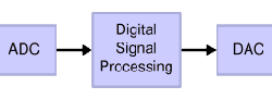
Category Archives: DSP Lessons

I am not going to analyse what DSP processors are different from regular microcontrollers as there are many differences that allow to boost performance in many specific tasks like filtering, FFT, etc. One thing is obvious that DSP processors have to perform mathematical calculations rapidly enough to get predictive results. Better result we want – more processing power wee need. We know that MCU are performing two main tasks: data manipulation and mathematical operations. But fact is that it has to be done really fast. General purpose microcontrollers aren’t optimised to perform these tasks effectively as microcontroller has to as much universal as possible to fit in many areas. In other words flexibility reduces performance.

DSP processors are more specialized microprocessors that ara optimised for tas that they usually do – multiplication and addition. Lets take most common DSP routine FIR digital filter implementation. It takes several samples of signal x[] and produces output signal y[] which is modified by multiplying appropriate samples by coefficients a_n .

y[n] = a₀x[n]+a₁x[n-1]+…+a_kx[n-k]

Continue reading →

One of frequently used signal characteristics are energy and power. In signal theory these therms require additional comments because they are a bit different from these what we are used to use in AC or DC systems.

What is power and energy? If wee connect R resistor to voltage U, then resistor will dissipate some power which is equal P=U²/R. During time T the energy loss on this resistor will be: E= TU²/R.

Now lets say that we ad some signal s() instead of DC voltage. In this case the power will depend on time as signal is time dependant. The therm is called instantaneous power: p(s)=s(t)²/R

in order to calculate energy loss during time T wee need to integrate:

Sometimes its is more convenient to calculate average power during some time T:

When talking about signal power we don’t care about R load. Therm Signal power usually is used for comparing different signals. For this it is agreed to use R=1, then we exclude resistance from formulation and then wee can talk about signal power and energy in signal theory:

Signal e3nergy may be finite and infinite. For instance finite signal will have finite length energy while its level wont go to infinite. Any periodical signal has infinite energy. If signal energy is infinite, then we can only talk about average power over all time axis:

Square root of average power gives root mean square (RMS) of signal:

Well for signals with period T you don’t have to calculate average power or RMS using lim function. This is enough to calculate average values during one period.

Sampling is a process when continuous time signal is represented by series of discrete samples while reconstruction is reverse process when these samples re recreating adequate continuous time signal. Bellow the overall process is illustrated.

Sampling is a process when continuous time signal is recorded every T seconds by multiplying by an impulse train.

If signal is sampled in frequency domain. For this we need signal transformed in to frequency domain. The frequency spectrum has to be band-limited. The impulse train after transformation becomes impulse train with scale in heigh 1/T. Multiplication in time domain becomes a convolution in frequency domain. After convolving the signal is scaled and shifted. The signal in frequency domain becomes periodical.

In order to reconstruct the signal x(t) from sampled spectrum first we need to extract the original spectrum. For this ideal filter is needed to take single spectrum from spectrum signal train. Low pass filter fill cut other copies of spectrum. The filter should have cut off at f=±1/(2T) and Gain of T:

After this reconstruction can be done. Ideal filter in frequency domain is a sinc function in time domain. This means that multiplying spectra by box in frequency domains means convolving with a sinc function in time domain. Because y(t) is a series of impulses, then reconstructed x(t) is a superposition of scaled and shifted sincs:

The fundamental result is that any band-limited signal can be completely discretized by equally spaced samples. And remember that sampling frequency has to be at least two times bigger than bandlimit of signal to avoid alias (overlap) of sampled signal spectra. Otherwise reconstruction of original signal becomes impossible.

In previous post we discussed about impulse response. Impulse response h(n) is digital system response in time domain. But there is another characterization of discrete system – frequency response H(e^jω).

Frequency response can be calculated form impulse response by formula:

where |H(e^jω)| – is amplitude frequency response

– phase frequency response.

There are two simple ways to calculate frequency response of discrete system:

First mentioned above – from impulse response;

Second – from discrete system equation:

Lets say we have digital filter described as:

y(n)=-a1·y(n-1)+b0·x(n)

then frequency response of digital filter would be: